“….no senior managers actually wanted to get their hands dirty and investigate the numbers.……..  they never dared ask me any basic questions, since they were afraid of looking stupid about not understanding futures and options.” – Nick Leeson, Rogue Trader

Since the beginning of 2025 Consilience has published two blogs:

• The first, “Oil Prices: When Does Complex become Too Complicated”, described how oil prices are agreed, focusing on the oil price negotiation that takes place when oil cargoes change hands. It explained that, when the composition of a published oil price benchmark changes, the price differential to the benchmark in contracts for non-benchmark oil has to be reviewed;
• The second, “Spoiled for Choice”, explored the value of options, or choices, given to an oil major or large trading company by a non-trading exploration and production (“E&P”) company or small refiner/consumer without its own trading capability. It considered how much such optionality in the contract price formula is worth from the perspective of the non-trading option grantor.

This third blog will look at the value of oil price optionality in a non-benchmark contract price formula from the perspective of the larger oil or trading company. It might be expected that, if the smaller non-trading company understands how much its trading counterparty is making, that should go some way to wresting a bigger share of the economic rent accruing to the trader from the option- right? Alas, it is not that simple. 

As we said in “Spoiled for Choice”, “It should be understood that as between the two counterparties to the physical sale and purchase agreement, the size of the option premium is a zero-sum game. However, the more active trading company is unlikely to be just buying the option to set the B/L date and the price averaging period and leaving it at that. It is likely that the cargo in question will form just one component of an arbitrage jigsaw puzzle, which will involve, in all probability, a number of financial and operational risks that must be hedged.” arbitrage jigsaw puzzle, which will involve, in all probability, a number of financial and operational risks that must be hedged.”

The Long and the Short of it

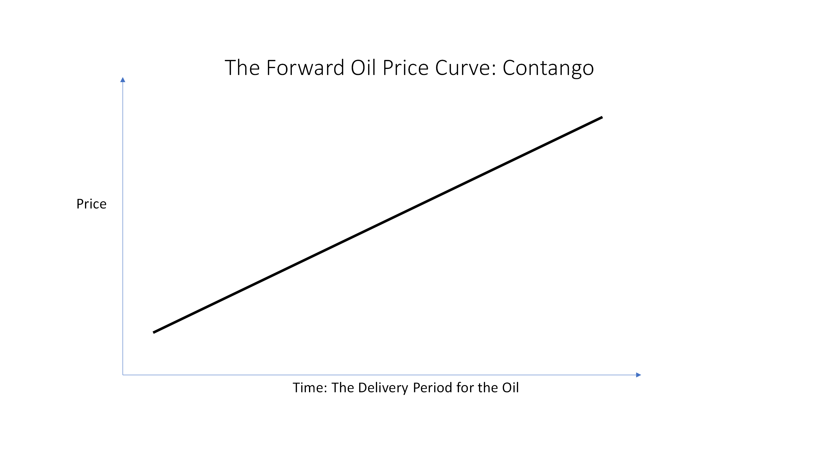
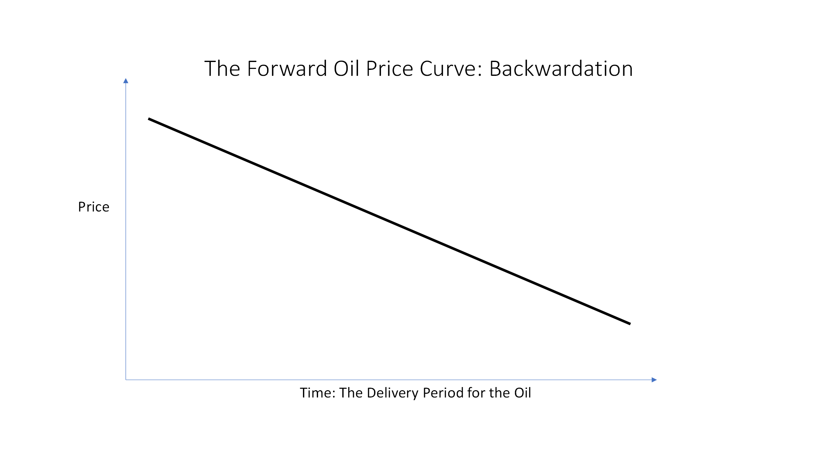
There is a widely held view that traders are gamblers who make their money from outguessing the next move in market prices. This may be a move in the height of the forward oil price curve (“A”), or the slope of the price curve, (“T”), as explained in our previous blogs. 

It is believed by some that traders buy, i.e., go “long”, of a commodity or asset and wait for the price to rise so that they can sell it for a profit. In other words, buy low, sell high. Or they may go “short”, i.e., sell a commodity or asset for forward delivery that they have not yet acquired in expectation of falling prices. They expect to cover their short position by buying in before they have to deliver the physical commodity. In other words, sell high, buy low.

This form of speculative activity is just one arrow in the quiver of a trading company, but not necessarily the sharpest, or most regularly used, one. It is capital intensive and very risky, particularly in a geopolitical and volatile commodity like oil. It is written on the gravestones of various speculative trading companies: “We bought high and sold low. Doh!”

Trading businesses are more likely to rely on arbitrage opportunities for their bread and butter, rather than naked speculation.  

Arbitrage

Arbitrage is the act of profiting by discrepancies in prices due to, for example,

• imperfect knowledge;
• location;
• illiquidity;
• seasonality;
• different product specifications in different regions;
• different environmental regulation in different regions;
• slow communication of new information; or,
• any other reason, such as the inability of two counterparties to deal with each other directly and therefore needing to insert a “sleeve” company into the chain of supply.

Usually, price imperfections are small and transient, because traders quickly recognise and exploit any such inconsistencies. Traders will sell those prices, or price components, that are over-valued, driving the price down, and buy those price components that are undervalued, driving the price up, so that they rapidly come back into an economically consistent line.

Examples of Arbitrage

Location: If the price of a product is different between two locations in the world, the trader may buy in the cheaper location and sell in the more expensive location. This activity continues until the cost of freight and the time value of money make it uneconomic.

Timing: If the price of oil for delivery in the near future is less than the price of oil for delivery in a later period (contango), the trader may buy oil and take delivery now and sell it for delivery later. This activity continues until the cost of storage and the time value of money make it uneconomic.

Quality: If the price of one specification of a product is lower than the price of a different specification of the same or a similar product, the trader may buy the cheaper oil and blend it to the specification of the more expensive product. This activity continues until the cost of blending components, freight, storage and the time value of money make it uneconomic.

Arbitrage is not risk free. The purchase and sales prices or price formulae have to be hedged. Otherwise, the arbitrage gain can be lost in a movement in the absolute price, A, or the time differential, T. This can be trickier in the case of a quality arbitrage because of the seasonal changes in product demand and specifications, and the blunter hedging tools available in the refined products market than in the crude oil market.

Illustrative Example

Readers whose day job is not trading may find it unnecessary to slog through the following example. We at Consilience have often found it helpful to work through some examples like this with industrial company board members, audit committees, regulators and judges/arbitrators in disputes to demystify the trading game. The explanation below is somewhat detailed and turgid, but it is not intellectually challenging. Those with a more superficial interest may wish to skip forward to the heading “Shooting at a Moving Target: Bullets are Costly”.

Using an old copy of Platts from 13th February 2024, (See extracts below) here's how it might work in one scenario:

On 13th February 2024, a third-party oil seller, which we will call (“Explorer”), agrees to sell a cargo to a trader, which we will call (“Trader”) for delivery in four weeks’ time. Four weeks forward from 13th February is the working week of 4-8th March 2024. The parties may agree to deem the bill of lading (“B/L”) date in advance as, say, 6th March. We discussed deeming in our previous blog.

To illustrate the issues, we will assume that the physical oil contract price formula that has been agreed is, say, the 2-1-2 average of Platts Dated Brent published on the 5 days around the B/L date +/- a grade differential, which we are calling “G”, as in previous blogs. G accounts for any differences between the Platts assessment parameters of Dated Brent and the characteristics of the physical oil in question.

The price component, G, is not easily hedgeable and is the most rigorously negotiated component of the price formula. It is where the Trader hopes to capture a profit. But in pursuing this profit, the Trader must ensure that any gain it makes on G is not lost in movements in the the slope of that curve, T, between 13th February when it buys the cargo from the Explorer and some later date when it sells the cargo to an as yet unknown third party on as yet unknown terms or in the height of the forward oil price curve, A, after 4-8th March. The components A and T were described in the previous blog.

The Trader’s price exposure must now be hedged.

EXTRACT ONE

Source: Platts

Extract one shows, among other things, Platts current assessment on 13^th February of Dated Brent for delivery 10-30 days forward from 13^th February, and the simultaneous assessment of forward cash Brent for delivery in M1, which is April, M2, which is May and M3, which is June. 

The report shows a “bid-offer spread”, i.e., the price bid by the best buyer and the price offered by the best seller, at market on close when the PRAs make their assessments. It also shows the midpoint of that bid-offer range as an assessment of the likely price that would be agreed if a deal was actually to be transacted. 

As we pointed out in our first blog “Often it is not actual deals negotiated and finalised in a contract that form the benchmark database for each grade of oil. It is frequently just price indications to buy or sell that do not result in an actual deal. And those deals and indications are those submitted to a price reporting agency (“PRA”) during a specific 15-minute period on an electronic platform each day. Only those companies that have been pre-approved by the PRA are permitted to input price indications to the PRA’s electronic platform. “

Extract Two shows Platts’ assessments of CFDs up to 8 weeks forward expressed as the Dated Brent differential to its own M2 Brent cash contract quotation. In reality, the CFD market trades up to 12 weeks forward expressed as a Dated Brent differential to M1, M2 or M3 as the two counterparties to any deal might agree.

EXTRACT TWO

Source: Platts

As mentioned above, although the PRAs publish CFD assessments up to 8 weeks forward from the publication date, the market trades up to 12 weeks forward, albeit in progressively lower volumes. Brokers can be consulted to obtain quotes for these further forward weeks, but a rough, back of the envelope assessment can be obtained by extrapolating the difference between CFD Week 7 and CFD Week 8. So, for example, CFD Week 9, namely 8-12^th April, on 13^th February may be estimated as May cash Brent minus $0.30/bbl, i.e.,  (($0.06-0.12)-0.12)) =-$0.30/bbl.

CFD Weeks 1 to 12 are separate contracts.These refer to the current value on 13^th February of the average difference between Dated Brent and the month 2, M2, forward cash Brent contract,which is to be published in each day of delivery Week 1, 12^th-16^th February, delivery Week 2, 19^th-23^rd February etc. These are expressed as a price premium or discount to the M2 cash Brent contract for the delivery week in question.

Some care must be taken when trading CFDs, particularly in the later weeks. This is because if, say, a Week 9 CFD is expressed as a differential to the May M2 Brent cash contract when it is purchased on 13^th February, it will cash settle by reference to the Dated Brent minus May Brent differential as published by the PRA during Week 9, i.e., 8-12^th April. However, by the time a Week 9 CFD comes to cash settle, the May cash contract will no longer be assessed by the PRAs and the May futures contract will have expired. So, a hedge of a late week CFD on 13^th February may have to be managed by rolling the May component forward to June at some point before the physical sales price averages out. We will show how this may be done later in this narrative.

Published price data, futures contracts and broker quotations allow us to construct a detailed forward oil price curve showing the value of oil for delivery on very precise future time periods. Chart One shows the forward oil price curve suggested by Platts data on 13^th February. The curve is showing pronounced backwardation, as discussed in our last blog.

Chart One: The Forward Oil Price Curve on 13th February 2024.

Source: Derived from Platts Extracts One and Two above

In our illustrative example of a sale and purchase contract for oil for delivery on a deemed B/L date of 6^th March, with the price averaging period being the 5 days around the deemed B/L date, i.e., 2-1-2 pricing, the value of the contract on 13^th February according to Platts assessments is: 

• May cash Brent $82.42/bbl; plus,
• CFD Week 4, $1.37/bbl; plus/minus,
• G.

This is equivalent to $83.79 +/- G/bbl.  This information is transient and is only useful if the Trader acts upon it. The actual contract price on the invoice that the Explorer sends to the Trader in due course will be based on actual published prices averaged over 4-8^th March.

So, on 13^th February, the Traderis now long of, i.e., committed to buy, a physical cargo for delivery on a deemed B/L of 6^th March based on Dated Brent averaged over the 4-8^th March, as published by Platts, +/- G.   The Trader may only have got itself into this position because it could identify an arbitrage opportunity, or in its judgement the likelihood of an arbitrage opportunity, to make a profit on the value of G by using one of the arbitrage strategies identified above. For clarity we will label the value of G in the Trader’s purchase contract from the Explorer as G1.

Armed with this explanation of the data available, for illustrative purposes we will assume a locational arbitrage where the cargo may be delivered in a later period to a different location where the value of G is sufficiently higher to cover the negative impact of backwardation, the cost of freight and the time value of money. We will label the value of G in the Trader ‘s onward sales contract to a refiner as G2.

So, on or after 13^th February, the Trader may sell the cargo perhaps to a refining company, which we will dub (“Refiner”). This may be a contract for delivery, say, 1^st -3^rd April, with a deemed discharge date of, perhaps, 2^nd April with Dated Brent pricing averaged over 5 days after the deemed discharge date. That would be the Platts publication dates of 3-9^th April 2024.

Already this is looking like a tricky deal.The market is in backwardation so, since the act of transporting the oil to a different geographic region takes time, the current market for later- delivered oil is already significantly below oil for delivery nearer term. Based on the values of A+T for 4-8^th March 2024 and for 3^rd-9^th April 2024 alone, this is a loss-making deal. So, to proceed, the Trader must have a reasonable expectation that the value of G2 will be greater than G1 by at least the extent of backwardation and must also compensate for the cost of freight and the time value of money.

While the Trader is focusing on arbitraging the value of G, elsewhere the height, A, and the slope, T, of the oil price curve are in constant motion and do not maintain the values that the Trader identified when it decided to proceed with the arbitrage on 13^th February. If the height of the curve, A, falls and/or the slope of the curve, T, rises between 4-8^th March, when the Trader’s purchase price averages out and by 3-9^th April, when the Trader’s sales price averages out, the Trader’s anticipated profit, G2 minus G1, may be diminished or eliminated.

If the Trader judges that the arbitrage was worthwhile on 13^th February, it would make sense to lock in the value of T that was apparent on 13th February, and the value of A that emerges 4-8^th March, lest they move against the arbitrage profit. There are various ways that both A and T maybe hedged if the Trader does not intend to speculate on their values in this, its long physical position.

Hedging

The Trader is at risk if the purchase price of Dated Brent 4-8^th March +G1 turns out to be higher than the sales price of Dated Brent 3-9^th April +G2 + cost of freight + the time value of money. On 13^th February Trader is probably making money on this deal on a mark-to-market basis, or it would not do the deal. Or the Trader may consider that it is worth taking a speculative risk even if a profit is not obvious on 13^th February because it may judge that the market will move in its favour.

But we will assume for illustrative purposes that the Trader identifies a profit on 13^th February and wishes to lock in that profit. It must now, on 13^th February, hedge the values of the difference between CFD Week 4-8^th March and CFD Week 3-9^th April. To do this it must:

• Hedge 1: Buy CFD Week 4, 4-8^th March, at M2 cash Brent, May,plus $1.37/bbl;
• Hedge 2: Sell three fifths of CFD Week 8 and two fifths of CFD Week 9, 3-9^th April, at M2 cash Brent, May, minus $0.19/bbl (i.e., 3/5 times -$0.12 plus 2/5 times -$0.30= - $0.19/bbl)

Hedge 1 will cash settle automatically by the Trader, in effect, selling back the average Dated Brent v May Brent differential as published by the PRA over 4-8th March. It is mostly irrelevant to the Trader’s overall arbitrage profit what the value of the Dated Brent average turns out to be: it may be higher or lower than the fixed value at which the CFD was purchased on 13th February, i.e., May Brent plus $1.37/bbl. This is because the hedge sale cash settlement price will mirror and cancel out the Dated Brent component of the physical cash purchase price between the Explorer and the Trader.

Hedge 2 would cash settle automatically by the Trader, in effect, buying back the average Dated Brent v May Brent differential as published by the PRA over 3-9th April. However, there is a catch attributable to the May contract expiry date. This will be explained in the next section of this blog. It is again mostly irrelevant to the Trader’s overall arbitrage profit what the value of the Dated Brent v forward cash Brent average actually turns out to be: it may be higher or lower than the fixed value at which the CFD was sold on 13th February, i.e., May Brent minus $0.19/bbl. This is because the hedge purchase cash settlement price will mirror and cancel out the Dated Brent component of the physical cash sales price between the Trader and the Refiner.

It is likely that the Trader will choose the futures contract as its hedging tool, rather than the 30-Day BFOETM forward cash contract. The cash contract trades in cargo volumes for 700,000 bbls at at time, not 20% of an unspecified physical cargo volume. The futures contract trades at fixed volumes of 1,000 bbls at a time and is much more useful for precision hedging. The value of T, the slope of the curve, may be hedged using the Dated to Frontline (“DFL”) contract, the equivalent of the CFD contract but based on the differential between Dated Brent and the first futures contract, rather than Dated Brent and the M2 cash forward contract.

Roll Out the BBLs

As indicated above, the May Brent component of both these CFD hedges opens up a further risk: if the height of the forward oil price curve, A, as expressed by the price of May M2 cash Brent, falls between 4-8^th March and 3-9^th April, the Trader’s arbitrage outcome will be less than it expected on 13^th February when it was set up.

To protect itself from a fall in the height of the forward oil price curve, A, the Trader may sell the May futures contract over the five publication dates of 4-8 March, to cancel out the absolute price exposure, A, on its purchase contract from the Explorer. It will intend to buy back the May futures contract over the five publication dates of 3-9th April, to cancel out the absolute price exposure, A, on its sales contract to the Refiner.

However, the Trader cannot buy back a May futures contract 3-9^th April, because the May contract will have expired at the end of March.  So, at sometime before the end of March, the Trader will have to close its short May futures position by buying the cargo volume on or before the May contract expires and reopen a new short position in the following futures contract month of June.

• Hedge 3: Sell, i.e. go short, May futures over the 5 days of 4-8^th March, 20% of the cargo volume per day;
• Hedge 4: Buy back May futures on or before end March, 100% of the cargo volume;
• Hedge 5: Sell, i.e. go short, June futures on or before end March, 100% of the cargo volume;
• Hedge 6: Buy back June futures 3-9^th April, 20% of the cargo volume per day.

Now the Trader can buy back its short June futures position over the five publication dates of 3-9ᵗʰ April, to cancel out the absolute price exposure, A, on its sales contract to the Refiner.

Alternatively, on 13^th February, the Trader may have anticipated the need to close its hedge over 3-9^th April. Being well aware of the expiry date of the May futures contract, the Trader may on 13^th February have entered into its CFD Hedges 1 and 2 above based on the published price differential between Dated Brent and M3 cash Brent, June, rather than M2 cash Brent, May. The PRAs choose to publish CFD assessments based on the published price differential between Dated Brent and M2 cash Brent. But two counterparties may construct a CFD trade with whatever structure they both agree, including based on the published price differential between Dated Brent and M3 cash Brent.

In either case, the Trader is exposed inevitably to the May/June cash Brent price spread either on 13^th February, or on any of the dates between 13^th February and the expiry of the May futures contract that it chooses to roll forward its hedge of the absolute oil price, A.

It is mostly irrelevant to the Trader’s overall arbitrage profit what the outcome of its futures Brent contract purchases and sales turns out to be: it may make a profit or a loss on these hedges. If it makes a profit, it will be because the height of the forward oil price curve has fallen, and it is buying back its futures hedges at a lower price. But this gain will be offset by the loss it makes between its physical purchase from the Explorer and its sale to the Refiner.

Shooting at a Moving Target: Bullets are Costly

The preceding discussion describes one possible scenario where the Trader identifies an arbitrage opportunity on 13^th February that relies on its ability to agree a value of G2 that exceeds G1 by enough to cover backwardation and its other costs. That is unlikely to be the end of the story for the Trader_.

During all the time period from 13^th February, when the purchase contract from the Explorer is agreed, up until 1-3^rd April, when the cargo is delivered to the Refiner, the Trader will be on the look out to improve its profit estimate, G2-G1. Perhaps this might be by substituting a different cargo for delivery to the Refiner and delivering the Explorer’s cargo to a different location, perhaps co-loading with oil from a different source to improve its freight economics or blending a product in-tanker to meet different regional quality specifications.  

Each time the Trader changes its arbitrage strategy it has to undo its hedges that were appropriate for the first strategy and put new ones in place to suit its new strategy. This activity is not cost free. The Trader must cope with a bid-offer spread at the time of dealing, sometimes tying up its credit lines with swap providers, paying brokerage fees and the depositing initial margin and variation margin with a futures exchange. These margins are security deposits paid to the exchange’s clearing house to guarantee payment and performance.

If the Trader hedges its absolute price risk, A, using the futures contract, rather than the forward cash Brent contract applicable to the physical cargo, it will also suffer basis risk attributable to the fact that the futures and the forward contract do not trade at exactly identical prices. The difference is referred to as the Exchange for Physical (“EFP”) difference and can be up to 10 cents/bbl, but more often around 5 cents/bbl.

Furthermore, the Trader is using a fixed volume financial instrument, CFDs, DFLs or futures, to hedge a variable volume physical contract. Most physical seaborne cargoes have an operational tolerance of +/- 5-10%, which was originally established to give the Master of the tanker flexibility to adjust the trim of the vessel or to sail light-loaded for safety reasons. So, if the physical cargo volume varies from the base contract volume the Trader may be over-hedged or under-hedged.

This also presents an opportunity. This operational tolerance is often appropriated by the Trader who has chartered the tanker for commercial reasons.  If the Trader is making money on the hedge side of its profit/loss equation and therefore must be losing money on the physical cargo size of the equation, it can choose to load 5-10% less on the tanker carrying the physical cargo to boost its overall profit.

Herding Cats

Large oil companies and trading companies are likely to have many different deals in progress, often traded in different offices around the world. All of these deals may need to be hedged and re-hedged to reduce speculative risk. To defray their dealing costs, such companies will often centralise their risk management activity, as illustrated below.

So, instead of each individual trader or trading desk within a trading company entering the market each time it has a risk to hedge, each such trader will undertake its hedge with the company’s own Central Risk Management desk (“CRMD”), marking the hedge to market at the time each trader logs a deal with CRMD. That mark to market value is the hedge price recorded on the individual trader’s profit and loss account for the cargo it is hedging. What the CRMD does with the risk transferred to it by the individual trader is up to the risk manager.

This is one of the reasons it is so difficult, but not impossible, to bring hedge gains and losses into the calculation when assessing damages in a trading dispute. It requires extremely detailed enquiry into the trade capture software of the hedging company. It also requires drawing a ring fence around the P&L account of the trader entering into hedges with its own CRMD.

To manage overall corporate price risk the CRMD may look for internal offsets in-house before laying off the Trader’s risk in the market or deciding to transfer it to a central corporate speculative trading book. 

Trading is a capital-intensive activity, not often appropriate to the business models of companies like the Explorer and the Refiner. It is not a slam dunk opportunity for traders to print money.

Price Optionality

In the light of the foregoing brief and simplified example of how a trader might go about generating a profit, we can now turn to the main purpose of this blog. This is to assess how much a small producer or refining/consuming company should charge a large oil or trading company for the option to deem the B/L date or choose the price averaging period in a sale and purchase contract.

Looking back at Platts Extract Two above, it is immediately apparent that, on 13th February when the Trader agreed to buy the cargo from the Explorer with a deemed B/L date of 6th March and 2-1-2 pricing, the Dated Brent component of the cargo was worth $83.79/bbl at that moment in time, and only at that moment in time.

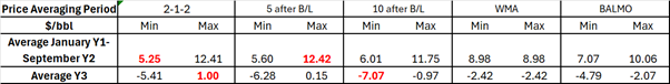
Had the parties agreed alternatively on 13th February, to deem the B/L date to be, say, 4th March with 2-1-2 pricing its value would have been $84.08/bbl. A deemed B/L date of 4th March and 5 after B/L pricing would give a cargo value of $83.67. Or, March whole month average (“WMA”) pricing for any March B/L date would give a cargo value on 13th February of $83.12/bbl.

So, as described in our blog, “Spoiled for Choice”, the default option in the oil purchase contract price formula is 2-1-2 pricing (the option market price) because that is what the cargo seller, the Explorer, prefers. The cargo buyer, the Trader, may want the option to choose 5 days after B/L pricing (the option strike price). That option has intrinsic value on 13th February. The deemed B/L date of 6th March was worth $83.79/bbl based on 2-1-2 pricing. But, on 13th February, the average of 5 days after deemed B/L of 6th March pricing was worth $83.42/bbl (i.e., 2/5 of week 4 and 3/5 of week 5). So, on 13th February, the option to change the pricing basis from 2-1-2 to 5 after B/L, had $0.37/bbl of intrinsic value. It can be said to be 37 cents/bbl in-the-money.

This might suggest that, if the Explorer is aware at all of the forward oil price curve on 13th February, it could seek an increase in the size of G1 by $0.37/bbl to account for the option’s intrinsic value. That is not going to happen. If the Trader is going to have to pay up to a $0.37/bbl higher grade differential, G1, for the option to choose between 2-1-2 and 5 after B/L pricing, the Trader might as well just trade the value of the difference between the two price averaging periods in the CFD market. This is a more liquid and more flexible way of trading the value of the time differential, T, than building optionality into a physical oil contract price formula.

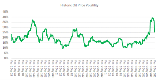
The forward oil price curve will give a different range of opportunities each day from 13th February up until the last day agreed between the Explorer and the Trader for the Trader to exercise its option to deem a different B/L date or a different price averaging period from the default price averaging period in the physical contract. The height and slope of the forward oil price curve are in constant motion and will offer different values for the absolute price, A, and the time differential, T, each day. If the market is volatile, the range of possible prices is likely to be measured in dollars rather than cents, as we illustrated in Table One in our blog “Spoiled for Choice”.

But as we said in this previous blog, hindsight is no guide to the future.

On 13th February the Trader may ask the Explorer for the option to choose the deemed B/L date or the price averaging period by, say, 1st March. It may ask for the right to opt for:

• 2-1-2 pricing, the default option in the contract; or,
• 5 after B/L pricing; or,
• 10 after B/L pricing;
• WMA pricing.

It will be recalled from the previous blog that the option premium is made up, not just of its intrinsic value, calculated as $0.37/bbl above, but of the time remaining until expiry, historic volatility, interest rates and implied volatility.

It is no simple matter to work out scientifically at what premium these so called “spread options” could have been traded in the market on 13^th February. It is certainly beyond the mathematical skill of the writer of this blog. Some form of Monte Carlo simulation is probably possible, but one of the problems is that there is no liquid market in non-standard options derived from a physical cargo contract. So, it is hard to get a fix on implied volatility. Hedging the price risk would be difficult, labour-intensive and costly.

In theory, if the Trader could agree a smaller increase in the size of G1 in its physical purchase oil price formula to acquire the option from the Explorer than the premium at which it can sell the option in the market to a third party, it could decide to sell the option. This is unlikely because there is no liquid market in these highly tailored options.

Furthermore, if the cargo purchased by the Trader from the Explorer is part of an arbitrage strategy, such as in the onward sale to the Refiner example above, the deemed B/L and price averaging period are very likely to be hedged, as described above. If that arbitrage depends on the size of G2 in its physical sales oil price formula with the Refiner being sufficiently bigger than G1 in its physical purchase oil price formula with the Explorer to cover its costs, then selling the option to choose the purchase price averaging period to a third party makes little sense. Apart from anything else it would leave the Trader with a difficulty in deciding which price averaging period to hedge in its contract purchase price formula from the Explorer: the choice would be out of the Traders’ hands and determined by the third party to whom the Trader had sold the option. 

Hence, deciding how much a small non-trading firm should charge a larger oil company or trader for the right to deem the B/L date or choose the price averaging period is not as simple as discovering the market value of the option on the day the deal is struck. However, the price negotiation will be less one-sided if the option grantor has established an appreciation of the practical shortcomings of any attempt to establish the theoretical option value at the outset. 

Clearly, bestowing such an option has a positive value, and as described in our last blog, the more volatile the market and the longer the larger trading company is given to exercise the option, the more favourable should be the option premium to the option grantor. 

As we said in our second blog, under the heading “Look Back in Anger”, granting a “look back” option is akin to letting your counterparty call heads or tails after the coin has landed. This will never work in the option grantor’s favour, so the grantor should be seeking a much, much higher premium if it sells this right. 

The option premium that the option grantor actually achieves depends mainly on how much muscle it can bring to bear in the negotiation. Trading is an art, not a science.

As we said in our first blog, the only way to ensure that small producers or refiners are getting the best price for their shareholders is for them to award a tender, always to a reliable company from as wide a range of counterparties as possible, that gives the most favourable differential to the tender price formula that is identical in every other respect. If one responder is seeking an option in the deemed B/L date or price averaging period and the others are not, the differentials are not comparable. 

If there is only one company, or very few companies, interested in the physical contract, then the scientific valuation of the pricing option is a moot point. There is no point in demanding a higher premium if your need to sell is imperative and there is only one buyer in town.  In the words of Dirty Harry: “...you've got to ask yourself one question: Do I feel lucky?' Well, do you, punk?"

The biggest difference between trading and gambling? In trading, the house doesn’t always win. Liz Bossley

Liz Bossley, with thanks to David Povey and Ben Holt for their help in peer reviewing this blog.

“When making a decision of minor importance, I have always found it advantageous to consider all the pros and cons.” – Sigmund Freud

In our last blog on 16^th January 2025 entitled “Oil Prices: When does “complex” become “too complicated””, we discussed all the moving parts that contribute to the oil price negotiating process. We talked about the choice of the most appropriate published benchmark price to use in a contract price formula and how the price differential to the benchmark has to change if the composition of the benchmark changes.

In that blog we said if a counterparty to a contract suggests that any form of optionality in the delivery dates or the price averaging period should be inserted into the physical contract price formula, then we enter new and even more complex territory. The purpose of this blog is to consider that issue. Readers whose day job is not trading may find it helpful to read the previous blog before embarking on a consideration of the impact of optionality in the oil contract price formula.

Time for T

One fact that the reader should keep front and centre in the mind is that the price of oil at any moment varies with its delivery date. The same barrel of oil can be worth simultaneously many dollars of difference in price depending on whether it is to be delivered next week, next month, or next quarter. This is not because oil prices are moving up and down all the time, although they are: it is because traders of oil will value identical oil at a higher or lower price today, depending on when it will be delivered.

Accordingly, the oil price formula in a contract will usually include a discount or premium to the chosen published benchmark price to reflect, among other things, any difference between the delivery date range of the cargo in question and the delivery date range considered by a price reporting agency (“PRA”) in assessing the benchmark price that the counterparties are using in their contract price formula. In other words, the contract should reflect any differences in the delivery date and pricing period of the contract oil compared with those of the published benchmark oil.

This concept is represented typically as a forward oil price curve, which is a graph showing the current market price, shown on the Y axis, for the same barrel to be delivered at various future points, shown on the X axis. The slope of the curve may be upward sloping from left to right (“contango”) or downward sloping from left to right (“backwardation”). This is illustrated in the Charts below. This is familiar territory to most oil executives.

In the first case, contango, oil for prompt delivery is less valuable at that point in time than oil for delivery in a later period.

Chart 1: Price Varies with the Delivery Date of the Oil- Contango

In the latter case, backwardation, oil for prompt delivery is more valuable at that point in time than oil for delivery in a later period.

Chart 2: Price Varies with the Delivery Date of the Oil- Backwardation

Both these charts represent a single point in time and what traders are prepared to pay at that point in time for oil to be delivered on different future delivery dates. It is not a price forecast.

The slope of the forward oil price curve can be referred to as the time differential (“T”) to distinguish it from the height of the forward oil price curve, the absolute price, determined by the benchmark price (“A”). The PRA publishing the benchmark price that the counterparties have chosen in their physical contract price formula, usually specifies the delivery date range it is assessing for a benchmark cargo. If the delivery date range of the physical cargo being negotiated is earlier or later than the PRA’s benchmark delivery date assumption, an adjustment in the contract price formula can be made in the form of a premium or discount to the benchmark price. This differential is derived from the slope of the forward oil price curve at the time of agreement.

The value of the time differential, T, can be fixed upfront by agreement by the counterparties to the deal, usually, but not always, at the time the physical oil sales contract is agreed.  This may be expressed as:

• minus $Z/bbl, indicating a contango market; or,
• plus $Z/bbl indicating a backwardated market.

The value of T, the time differential, like the benchmark price, A, is easily hedgable in the Brent market. In the case of the time differential, T, the hedging instruments available are the Dated-to-Paper contract for difference (“CFD”) market or the Dated-to-Frontline (“DFL”) markets.

Although “CFD” is a widely used term in the commodity markets simply meaning a swap, in the case of the oil market, CFD refers to the specific swap of a price differential between Dated Brent and, usually, the second contract month (“M2”) Forward Brent contract. These terms were explained in our blog of 16^th January 2025.

A nascent CFD market for WTI FOB Houston based on 10-day average pricing contract periods has now emerged and is reported by the PRA, Argus.

The Brent CFD market is widely used internationally to set the value of T in physical oil contract price formulae, or to hedge the value of T when traders are locking in a margin between the purchase price and the sales price of cargoes of many different grades of oil across the world. The practice of rolling CFDs when trading companies hedge the value of T will be explained in the next blog.

It is not easy to understand that the “commodity” in question in a CFD trade is a just a price differential, which can be traded as easily as any other commodity. Once that concept is firmly fixed, the mechanics of the CFD market become quite straightforward. It is a simple swap. It establishes the traded value today of the time differential, T, the difference between the market price of oil for delivery 10-30 days forward from the publication date and the market price of oil for delivery at some future date, typically, but not exclusively, 2 months forward. CFD contracts in the oil market are usually arranged into separate contracts for weekly delivery periods up to 12 weeks forward.

• The trader may fix today the value of T for the delivery dates in, say, week 3 (i.e., 3 weeks forward from the date on which the contract is being negotiated) at, for example, $0.25/bbl;
• The trader will cash settle the swap based on the difference between $0.25/bbl today and the actual average published price differential between Dated Brent and Month 2, M2, forward cash Brent, as published later during week 3.

Bearing in mind the link between the delivery date of a cargo and its price, we can now consider the main purpose of this blog, which is to consider how small producers or refiners may wish to respond to proposals by larger oil companies or traders to build some form of optionality into a physical oil contract price formula.

The Secret of Prices: It’s All in the Timing

The sort of optionality we have in mind is, for example, when the buyer or seller of a cargo suggests that it should have the option to change the agreed delivery dates of a cargo or to shift the price averaging period of the benchmark price in the price formula.

It can be quite seductive if, say, the buyer proposes to pay the seller a better differential to the benchmark in return for the right to choose the delivery date or the benchmark price averaging period.  This may be couched in terms such as, for example, the price will be the buyer’s choice between:

• the average of benchmark prices published on the 5 days after the bill of lading (“B/L”) date plus a differential of $0.50/bbl; or,  
• the average of the benchmark prices published on the 10 days after the B/L date, plus a differential of $0.65/bbl.

Obviously, a seller wants a formula that delivers the highest price possible, and the buyer wants a formula that delivers the lowest price possible. But how can anon-trading company decide in advance, sometimes even before the loading date range of the cargo is confirmed, if the extra $0.15/bbl is sufficient compensation for ceding the right to choose the published price averaging period in the contract formula, or even to choose the B/L date itself?  The larger trading company probably a team valuing and hedging such options. The smaller industrial company probably does not.

The B/L Date: A Moveable Feast

Given the logistics of moving oil around the world in tankers, it is difficult to be certain in advance what the B/L date of any cargo will actually turn out to be. There may be loading or cargo documentation delays at a terminal. A ship may arrive early or late. The party in control of the tanker – the buyer in an FOB sale or the seller in a CFR, CIF or DAP sale- may decide to slow steam to ensure as late a B/L date as possible, or alternatively to order the “caps on backwards” speed to ensure as early a B/L date as possible. Because the ultimate price formula is calculated by reference to the B/L date, unsurprisingly there is a temptation to tweak the dates. This is particularly so around the month end when there may be a change in the host government’s Official Selling Price (“OSP”) for taxation, cost recovery and profit-sharing purposes between the months.

Often, to provide certainty and to facilitate hedging, the parties will “deem” the B/L date in advance. In other words, they set a likely B/L date and use that date in the contract price formula irrespective of what the actual B/L date turns out to be. It is not unusual for the party pushing for a deemed date to be the bigger of the two oil companies or the entrepreneurial trading company on one side of the deal. This is because such, more trading-orientated, companies will be considering a range of possible strategies for the cargo, which will require hedging their price risk to lock in the margin that they have identified in advance of loading, often at the time the deal is struck.

So, in summary, because the calculated outcome of the contract price formula varies with the B/L date, if the B/L date is a movable feast, it is difficult to hedge the price risk. Agreeing to “deem” the B/L date in advance of loading can help the more active trader to manage its risk because it sets the apparent B/L date in stone, irrespective of what it actually turns out to be.

Cui Bono?

Exactly how the larger and more trading-orientated counterparty of the two is probably arbitraging the cargo and earning a profit will be the subject of a subsequent blog. The trading company will typically be taking every decision with the forward oil price curve as a constant companion. This is less likely to be the case for a small exploration and production (“E&P”) company or a small refiner/consumer.

Typically, a small E&P company or a small oil refiner/ consumer has no interest in, or capability to pursue, the trading opportunities exploited by its larger counterparty. It may well have a completely different business model and make its money from activities in which the larger trader may have limited or no interest, such as finding oil with a drill bit or by upgrading and blending hydrocarbons in a refinery or storage tank.

Hence, it may make sense for the smaller company to sell the trading opportunities that the inclusion of optionality in the oil contract price formula represents. If a company is not going to exploit that optionality itself, it might as well sell it and get some value from having the option in the first place by virtue of owning oil production or owning a refinery or blending facility:  the “use it or lose it” principle.

But a word of warning: the grantor, or seller, of the right to choose should be aware of the tax reference price(“TRP”) or Official Selling Price (“OSP”) it will face when it reports to the relevant Tax Revenue Authorities or government custodian of the Production Sharing Contract or Service agreement. This may be based on the actual B/L date and the taxation or other government authority may not recognise the deemed B/L date that sets the physical contract price. This will give the option grantor hidden basis risk.

Buying an option of any kind in a commodity or financial instrument is a risk-reducing activity. Selling an option is a risk-increasing activity. So, if a small producer or refiner grants, or sells, the option to choose the delivery date or the price averaging period in the oil contract price formula, it is advisable to have a good understanding of the risk it is taking on and the value of that risk, or option, in the market.

Options 101

The value of the option to choose, or deem, the B/L date and/or the benchmark price averaging is straightforward Options 101. The value of any choice, or option, is determined by:

• the current market price for the relevant period;
• the strike price;
• the time remaining until the option expires;
• historic volatility of the oil price;
• interest rates; and,
• implied volatility.

Options traders have a mathematically complex model that allows them to calculate the price of an option, referred to as the options premium, based on variations of the Black Scholes options valuation model. The variables listed above are variables in the Black Scholes model.

There are three basic types of option, which have a range of different labels in different commodities and in different areas of the world. For the purposes of this blog, we will use:

• European style options, which can only be exercised on their expiry date;
• American style options, which can be exercised at any time up to and including the expiry date;
• Asian style options, which cash settle automatically based on an average of benchmark prices published on a number of future dates that are specified at the time the option is negotiated.

In the case of oil, usually contracts between a non-trading firm and an oil major or trading company involve Asian style options. This is because, in such contracts, the price formula is usually an average of benchmark prices published over a number of days, rather than a single number, $X/bbl.

It may not be immediately obvious how these concepts apply in the case of granting an option to deem the delivery date or choose the contract formula price averaging period, but they do.

Market Price and Strike Price in an Asian Style option

For the purpose of this blog, to value what the right to choose or change the B/L date or the price averaging period, a bit of imagination is needed. It needs the reader to put themselves in the shoes of the option seller without its own trading department.

The strike price of any option may be identified as the price that the recipient of the option is acquiring the right to choose. If that strike price is more favourable than the current market price then the option is said to have intrinsic value, or to be “in-the-money”. It has a positive value. The opposite case is when the strike price is less favourable than the current market price and the option is “out-of-the-money”. It has no intrinsic value.

These terms mean simply that if you were to exercise the option now would you be making or losing money. If an option is losing money, it will not be exercised and will expire worthless. Alternatively, it may be sold in the market to recover that part of the option value that is not associated with the difference between the strike price and the current market price, as described above.

 In the context of this blog, consider the strike price to be the right to choose alternative contract price formulae that the grantor, or giver or seller, of the option is giving its counterparty. Whether the option can be said to be in or out-of-the- money will depend on a comparison of the strike price formula compared with the current benchmark market price of the “correct” price formula for the cargo in question. This is where it gets interesting. What is the “correct” benchmark price averaging period of any cargo?

As we said in our previous blog of 16^th January 2025, Platts assumes that, in the case of North Sea grades, contract price formulae often use the 5-day average of published prices around the B/L date for physical oil, with the B/L date being the mid-point of the price averaging period. This is so-called “2-1-2” pricing. In the case of West African grades, the norm is to use the 5-day average of published prices after the B/L.

Not all actual deals done in the market are transacted on a 5-day average period, particularly in the case of refined products.  This is just what Platts assumes in assessing oil prices for publication purposes. Some deals are done on a whole month average (“WMA”) price, with the month being determined either by the actual B/L date, a deemed B/L date or the date of the Notice of Readiness (“NOR”) to load or discharge the cargo. Others are done on a balance of month average (“BALMO”).

So, when it comes to evaluating the intrinsic value of an option to choose the contract formula price averaging period or to deem the B/L date, what is the correct benchmark price averaging period of any cargo? This is what will take on the role of “market price” in establishing the intrinsic value of the option in our analogy.

The practical answer is that the de facto market price is whatever the grantor of the option wants it to be. If the smaller company wants 2-1-2 pricing that is the de facto market price. If the larger company wants the option to choose the average of published prices published on the 10 days after the deemed B/L date that becomes the de facto strike price.

So to be clear, if, say, a small producer enters into a term contract to sell its oil it might prefer that for each cargo delivered under the terms of a long-term contract the formula contract price will be based on, for example, the WMA of published benchmark prices over the month in which the B/L date of each cargo falls, either actual or deemed. That can be considered to be the market price for option evaluation purposes in the context we are considering in this blog. If the counterparty would like to option to choose a different price averaging period or deemed B/L date, that alternative price becomes, in effect, the strike price of the option.

What You See Depends on where You Stand

From the perspective of the larger, trader-orientated company, the option can be considered by reference to the forward oil price curve and the CFD market. This will be discussed in our next blog.

From the perspective of the smaller producer or refiner, the forward oil price curve may be unfamiliar territory and too remote to assist in working out the ex-ante value of giving away the choice of B/L date or price averaging period. Such companies, understandably, often value the option ex-post. In other words, they are only concerned with the price in $/bbl that emerges on the invoice after the prices for the contract price formula chosen by the larger company have been published by the PRA.

When the contract is being negotiated, the smaller, less trading-savvy, company may evaluate the option by looking at what price the various alternative contract formulae would have delivered historically. This will suggest a completely different option value than the one available to the larger, more trading-orientated, company derived from consulting the forward oil price curve and their option valuation model at the time of the contract negotiation.

This is a fundamental philosophical difference in approach between small “industrial” firms without their own trading department and large oil and trading companies.

As mentioned above, we will consider the traders’ approach to this issue in our next blog. But the ensuing discussion looks at the issue from the perspective of a small E&P or refining company wanting respectively the highest or lowest price possible.

Illustrative example

In attempting to illustrate the issues associated with optionality we have considered actual prices during a typical historic 3-year period, Year 1 (“Y1”), Year 2 (“Y2”) and Year 3 (“Y3”).

Suppose that in October of Y2, a small E&P company was lining up a contract to sell 1 cargo per month in the following year, Y3. Having agreed which benchmark to apply, the E&P company has to decide which price averaging period it will agree with a buyer to use for each cargo in all the months of the delivery year, Y3.

One starting point might be to look at what the various likely price averaging periods might have delivered in the previous two years, Y1 and Y2. [Note:  At this point in the narrative, we are only considering the benchmark price averaging period for A, not the time differential, T, or the grade differential, G.]

In October Y2 an analysis of the previous Y1 and year- to -date Y2 would show that, compared with a fixed index, with hindsight we can say that the 5 after B/L price averaging period could potentially have yielded the highest price on average for each month and that the 2-1-2 price averaging period could have yielded the lowest price (See Table One).

The price outcome from different price averaging periods depends on the actual or deemed B/L date of each cargo delivered each month. Hence there is actually a Min-Max range of outcomes for each price averaging period.

Table One: Historic Analysis of Price Averaging Periods

It is evident from Table One above that the range of possible price outcomes from different price averaging periods not only depends on the actual or deemed B/L date but that it may be measured in dollars, not just a few cents. This should be borne in mind when selling the option to choose the price averaging period or the B/L date.

The small E&P company seller, in the absence of information concerning the forward oil price curve in October Y2, might have decided to take the middle road and go for whole month average, WMA, pricing. This would eliminate the range of different possible outcomes for each price averaging period arising from the movable B/L date. It would also iron out the peaks and troughs in the market value of benchmark price, A, applying to its possibly sole cargo each month. This becomes the seller’s preferred market price for the purpose of the option valuation discussion.

Had the E&P seller chosen WMA pricing, by looking back when it got to the end of Y3 it is apparent that the absolute price, A, had fallen substantially. Choosing the WMA pricing period would have delivered an average price outcome in the middle of the range of possible average price results.

That is all that this form of historic analysis reveals. It is an inadequate basis on which to choose the “best” price averaging period going forward, other than possibly leaning towards as long a price averaging period as possible.

The forward oil price curve in October Y2 would have shown the price, in October Y2, at which oil could be sold for delivery in each of the months of Y3. The E&P company could then have chosen to lock in the forward oil price curve value of A, the benchmark, by hedging.

Small consumers and E&P companies do not always consult the forward oil price curve or have the financial capacity, or board delegated authority, to hedge. Unless a company decides to act on the forward oil price curve now by hedging, today’s curve becomes no more than the white noise in the market, and it will have changed by tomorrow.

The forward oil price curve is the territory in which larger oil companies or trading companies mine for profits. As mentioned above, the traders’ approach will be explored in the next blog. Suffice to say for the purpose of this blog that the profit opportunities enjoyed by trading companies will often prompt them to seek the option to choose from two or more price averaging periods or deemed B/L dates in a sale and purchase agreement with a non-trading company. These alternative pricing and deemed delivery date proposals are analogous to different option strike prices to the non-trading company.

If the non-trading company is not in the position to exploit such profit opportunities, it makes considerable sense to sell this flexibility to someone who can. But at what price should the option to choose from two or more price averaging periods or deemed B/L dates, be sold? That depends on when the option has to be exercised and how long the buyer of the option has to decide which of the alternatives to choose. This is the option’s time to expiry.

Time to Expiry: Look Back in Anger

The time element of option valuation refers to how long the buyer of the option is given to decide whether or not to exercise the option before it expires. The more decision time allowed until expiry and the nearer is the expiry date to the contract price averaging period, the more expensive the option. This is because the longer the option buyer has to decide the more likely it is that natural market price movements will put the option in-the-money. The nearer is the exercise expiry to the beginning of the price averaging period, the more data the holder of the option has to inform its choice.

Ideally, from the seller’s viewpoint, the option should expire just before the price discovery period starts. So, if the option is to choose between, say, 2-1-2 pricing and 5 after B/L pricing, the option might best expire 3 days before the B/L date, when no information is yet available on what price of benchmark, A, will be published for each of the dates in question. Similarly for WMA pricing for month, M, the option expiry might best be set at the last day of M-1.

But the less time the option buyer is allowed, the less valuable the option and the less the option buyer will be prepared to pay. This is a risk/reward trade-off for the option seller.

It is becoming increasingly common for traders to seek “look back” options, i.e., the right to choose the price averaging period or the deemed B/L after all the relevant prices have been published. This is equivalent to having the right to choose heads or tails after the coin has landed. So, the option buyer, logically, will always choose the price most favourable to itself each month, to the detriment of the option grantor. It will never act in favour of the option grantor.

Traders or large oil companies may well offer seemingly attractive price differentials to have a look back option, perhaps $0.50/bbl or more. But a quick recap of Table one above indicates that a look back option can cost the option seller many dollars of lost revenue, or opportunity cost, on average each month.

The actual impact of the look back option is to give the seller the least favourable price on each possible B/L date, not just on average each month, so the opportunity cost can be much greater than the monthly average price implies.

The option grantor may decide to agree to a look back option anyway, gambling that the market will be calm and the difference between the highest and lowest possible price outcomes that it is foregoing will be less than the gain it makes from the better price differential in its sale and purchase contract for the oil. The more volatile is the market, the greater the gamble.

Historic Volatility

Volatility is one of the variables that options traders consider when valuing the price of an option. The more volatile is the market the more likely it is that the option will become “in-the-money” even for a short period of time and allow the option holder, or buyer, to exercise it, or sell it, at a profit.

When there is an event or an announcement that has an impact in the price of oil there can be a sharp spike in volatility, triggering the exercise, or sale, of some options which have come into the money.

This is not a variable that has much meaning in a quantitative sense to a non-trading company, but it is of some relevance in the eyes of a trader. Even companies without an active trading department can observe whether or not the oil price has been volatile recently and judge subjectively if such volatility is likely to persist in the future.  High volatility is unlikely to act in favour of the option seller, unless they can extract a higher premium from the option buyer.

Chart 3: Historic Oil Price Volatility

Interest Rates

In basic economics, all investments are measured against the risk-free alternative, i.e., instead of writing an option, the option seller could put its money in the bank and earn interest. The higher the interest rate, the more an option grantor will want to compensate it for the risk of granting an option. So, the higher the interest rate, the higher the option premium.

Again, this is not a variable that is likely to enter into the thinking of a small E&P or refining company when deciding whether or not to allow the larger trading-orientated company the right to choose the price averaging period or the deemed B/L date in a sale and purchase contract.

Implied Volatility….. then take away the number you first thought of!

Implied volatility can be described as the level of volatility required to generate the option premium that is actually being traded in the market. Given a known market price for the underlying oil, a known option strike price, expiration date, historic market volatility and interest rate, the Black Scholes model may suggest a certain ”scientific” option premium. But if the same option is actually trading in the market at a different option premium, the difference can be referred to as “implied volatility”.  It is shorthand for all the other factors that have an influence on the price of the option. This simple description annoys the bejeezus out of pure options traders.

Implied Volatility is most likely to be heavily influenced by the bargaining strength of the two counterparties to the physical oil sale and purchase agreement and how much of the “economic rent” the buyer of the option is prepared to share with the seller of the option. It will be shaped by the number of other parties in the market competing to take the other side of the smaller company’s deal.

Negotiating the Option Premium

It would be naïve to expect that the foregoing analysis would be of much assistance to a non-trading company attempting to put an objectively” correct” price for giving away the right to deem the B/L or to choose the price averaging period. However, there are several messages to take away from this blog:

• Historic data on the relevant oil benchmark price is of very limited help in deciding which contract oil price formula would deliver the most favourable result in the future;
• If a company is selling the right to choose the contract price formula, it should check if the tax reference price or OSP that will be applied to its revenue by the taxation or other government authorities is different, to ensure that it will not be taxed on revenue it does not actually receive;
• Ceding to a third party the right to deem the B/L or to choose the price averaging period can result in more than just a few dollars/bbl of difference in the final price that appears on the cargo invoice and considerably more than a few cents/bbl;
• The longer that the third party is given to elect what the deemed B/L or price averaging period will be the greater the value of the option to that third party;
• Granting a “look back” option will never work in the option grantor’s favour, so the grantor should be seeking a hefty premium if it sells this right;
• The more volatile the market, the greater the value of the option;
• If interest rates are high, the option grantor might try to seek a higher option premium, but, in reality, this is not an influential variable in the negotiation of the contract price formula for physical cargoes;
• How much of the profit opportunities enjoyed by the trading counterparty it is prepared to share with the option grantor in the form of a higher premium will depend on the relative bargaining strength of the two parties and the extent of competition from other third parties to do the physical deal.

It should be understood that as between the two counterparties to the physical sale and purchase agreement, the size of the option premium is a zero-sum game. However, the more active trading company is unlikely to be just buying the option to set the B/L date and the price averaging period and leaving it at that. It is likely that the cargo in question will form just one component of an arbitrage jigsaw puzzle, which will involve, in all probability, a number of financial and operational risks that must be hedged.

Although industrial firms without a trading department might not be in a position to enjoy the profit opportunities available to a trading company, before agreeing a price to give them away, it would be helpful to understand the profit prospects available to active traders.

That will be the subject of our next blog.

Hindsight is no guide to the future.

“The farther back you can look, the farther forward you are likely to see.” ― Winston Churchill

Sorry, Winston, I disagree. Not if someone rearranges the landscape with tariffs, sanctions, production shutdowns, wars or some other fundamental game-changer.

I prefer: “The future is an undiscovered country”- Klingon Chancellor Gorkon (with apologies to Hamlet)

Liz Bossley, with thanks to David Povey and Ben Holt for their help in peer reviewing this blog.

"Everything is complicated; if that were not so, life and poetry and everything else would be a bore." Wallace Stevens

It is often trotted out that the “right” price of any good or service is the highest price at which a buyer will buy and the lowest price at which a seller will sell. That’s all very well, but if only one party, or in some cases, neither party understands the price they are agreeing who is to say that the price is fair or a true reflection of market forces?

This blog will give a brief chronicle of how oil prices are agreed, not from the perspective of the supply/demand balance and the absolute level of oil prices, but by focusing on the oil price negotiation that takes place when oil cargoes change hands. Traders know all about this but oil industry professionals who are not directly involved in trading may wish to skim the ensuing explanation. It is not necessary for those readers whose day job is not trading to absorb the minutiae of the price formation process. However, an appreciation of the complexity of all the moving parts that interlock in pursuit of a fair market price for oil is advisable.

Safe to say, if you wanted to design the perfect oil pricing mechanism, crude oil or refined products, you would not start from here. But here is where we are!

Formula Pricing

To recap, the oil market abandoned fixed pricing, such at $X per barrel (“$X/bbl”) or $X/tonne (“$X/Mt)”, in contracts for the majority of physical cargoes starting in the 1980s. Instead, we went to formula pricing which reflected the published price of one of the fixed benchmark contracts, such as forward Brent or Dubai or the futures contract in WTI, averaged over an agreed period of time plus/minus a differential to reflect the value of any differences between the benchmark price and the oil in question. The market for refined products followed suit on formula pricing, developing benchmarks from Rotterdam, New York Harbour, the US Gulf Coast and Singapore, amongst others. This is old news!

The important point is that benchmarks have at least one of their contracts that are traded at a transparent fixed price, $X/bbl or $X/Mt, that can be used to solve the oil price formula in non-benchmark contracts.

Non-benchmark contracts contain a formula that allows the trader to agree a differential, $Z/bbl or $Z/Mt, to the benchmark number $X/bbl or $X/Mt, where Z itself may be a formula that expresses a value for all the differences between the characteristics of the benchmark grade of oil and the characteristics of the grade of the non-benchmark grade of oil question. The value of $X/bbl or $X/Mt in a non-benchmark price formula is usually the published value of X, averaged over a number of days publications. To this value of X a price differential, $Z/bbl or $Z/Mt, is added or subtracted.

Maintaining the Benchmarks

That was all fine, so long as there were sufficient observed fixed price deals transacted to establish the standard benchmark price, X. This benchmark price, averaged over the pre-agreed period, was then plugged into the price formulae in non-benchmark, which we will call “physical”, oil contracts for convenience, to deliver a fixed price result for physical oil. This is the number that appears on the invoice, i.e. X+Z.

Over time the benchmarks have altered out of all recognition. Production of some benchmark grades of oil has declined, trade routes and delivery points have transformed in response to legislation, sanctions, shifting consumer demand and improvements in infrastructure and, particularly for refined products, tightening environmental regulations. Typical efficient cargo sizes (and therefore freight costs) have also evolved. If the characteristics of a benchmark, X, change, the formula price differential for physical contracts, Z, also has to change.

Often those negotiating physical contracts do not appreciate the, sometimes subtle, changes that are happening to the benchmarks and therefore fail to recognise that the formula price differential that has applied to their physical oil in the past has now to be adjusted for future cargoes.

The logical response to changes in the level of production of benchmark grades and therefore the number of transactions informing the published benchmark prices, might have been to allow the benchmarks to evolve too, some disappearing and new ones growing. If that had happened physical oil contract price formulae would have contained new benchmarks with price averaging periods and price differentials for physical grades reflecting departures from the new benchmark characteristics.

But that is not what has happened, particularly for crude oil benchmarks. Instead, the market has gone to extraordinary lengths in some cases to preserve the semblance of old benchmarks, such as Brent, which is discussed in some detail below. This benchmark has included more and increasingly disparate grades of oil from different locations into the benchmark price discovery database to shore up the old benchmark.

If a party to a physical oil contract does not understand what a changed benchmark, X, now represents and how it is compiled, how can it hope to agree a fair price differential, Z, in a physical cargo oil price formula?

Deal Data Underlying Benchmark Quotations

Often it is not actual deals negotiated and finalised in a contract that form the benchmark database for each grade of oil. It is frequently just price indications to buy or sell that do not result in an actual deal. And those deals and indications are those submitted to a price reporting agency (“PRA”) during a specific 15-minute period on an electronic platform each day. Only those companies that have been pre-approved by the PRA are permitted to input price indications to the PRA’s electronic platform.

The PRAs are at pains to consider other transactions not input directly to the electronic platform in arriving at a final published number. It is my understanding that the PRA considers all the information at its disposal, not just electronic platform data, and normalises non-standard transactions onto the same basis as the characteristics of its benchmark when it has sufficient data to do so.

What could possibly go wrong?

Basket Cases

A significant level of complexity arises when a price benchmark reflects the price of, not one specific grade of oil, but a basket of similar grades of oil, any of which can be delivered in satisfaction of a contract.

This is a predominantly crude oil phenomenon, rather than for refined products. This is because refined products are typically defined by their quality specifications rather than by a “brand name” that defines their origin. For refined products, baskets usually only arise for delivered (CFR, CIF, DAP etc.) transactions where the freight component of the price may involve a basket of possible origins for product delivered to the delivery point specified in the benchmark.

In the case of crude oil, a distinction must be drawn between a blend and a basket.

Many grades of crude oil are actually a blend of oil arising from many different oil fields that are gathered in a common pipeline or that are commingled and use shared storage and export facilities. The quality of blends can vary depending on the relative production rates of the different fields contributing to the blend.

Baskets are something different. Baskets are employed when a range of different crudes from different origins can be delivered in satisfaction of a contractual commitment. Examples of baskets include:

• A middle east crude (“MEC”) benchmark, which is the lowest price of a basket of Dubai, Oman, Upper Zakum, Al Shaheen and Murban;
• The Argus Sour Crude Index (“ASCI”), which is a basket calculated as the volume-weighted average of each day’s differential trades for Mars, Poseidon and Southern Green Canyon added to the WTI futures contracts first month settlement price; and,
• The Brent basket, which is by far the most pervasive and complex benchmark. It is perfect for a case study of the issues that arise when a basket benchmark is employed in physical oil contracts. It is therefore considered in some detail below.

The Brent Basket

In the case of the ubiquitous “Brent” benchmark, by now most actors in the oil industry have cottoned on to the fact that the price of Brent as published by the PRA, Platts, has very little to do with the Brent of old. It is now the lowest of the prices for a basket of grades including Brent, Forties, Oseberg, Ekofisk, Troll or, since June 2023, WTI Midland (“BFOETWTIM”).  Yes, West Texas Intermediate gathered at Midland Texas! We’ll come back to WTI later in this blog.

• Dated Brent: This refers to cargoes to which a 3-day loading date range has already been allocated by the relevant terminal operator. Only cargoes scheduled for delivery during the 10-30 days forward from the date of the publication in which the assessment is made are included in the published assessment. Dated Brent cargoes may be traded in the market with a shorter or longer lead time to delivery, but the published price assessment refers to cargoes for delivery 10-30 days forward.  The Dated Brent price is determined each day from the cheapest of the grades in the Brent basket. This market usually trades in cargo lots of 700,000 bbls to maintain fungibility with the forward cash market but may trade in whatever cargo size is agreed between the terminal operator and the producer owning the cargo.  
  
• Forward Brent, or cash Brent: the Brent forward contract, sometimes referred to as “cash” Brent, allows a buyer and seller to trade a Brent basket cargo for delivery at any time during a specified future month up to several years ahead. The seller must tell the buyer which of the grades in the Brent basket - Brent, Forties, Oseberg, Ekofisk, Troll or WTI- it will deliver and on which 3-day delivery date range in the specified month it will deliver it, by 30 days before the first day of that particular delivery date range being supplied. This market trades in cargo lots of 700,000 bbls.
  
• Futures Brent: This is Brent traded on a regulated futures exchange in cleared contract lots of 1,000 bbls. “Cleared” refers to the fact that the clearing house of the exchange requires an initial margin and a variation margin, i.e., deposit, from all contract holders, both buyers and sellers to ensure payment and performance by both sides of any transaction. Each contract is for Brent for delivery in a future month up to several years ahead. The underlying commodity is cash Brent. 1,000 bbls is not a deliverable quantity so these contracts tend to cash settle by the closing of positions before the expiry of the contract for the relevant month, M, by the last business day of M-2. However, any two parties may agree delivery of a cargo “off-exchange” and give this up to the exchange for clearing through an Exchange for Physicals (“EFP”) mechanism. This volume is reported by the exchange, but the price of the EFP is not recorded as a traded price by the exchange, because it has not been offered to other buyers and sellers on the exchange.
  
• Brent CFDs: This is a swaps market where the underlying commodity is the published price difference between Dated Brent and cash Brent. This is an over-the-counter (“OTC”) market in the price differential between Dated Brent for delivery 10-30 days forward and cash Brent for delivery in a forward month. Each contract expresses an assessment of what the published price differential between Dated Brent and cash Brent will be during each separate forward trading week, typically 8-12 weeks forward from the trading date. So, today traders may buy or sell Week 3 at, say, +$0.50/bbl. This contract will cash settle at the end of the actual Week 3 when all the published price data for Dated Brent and cash Brent for that week is known. The contract is a swap, so it can only cash settle: physical delivery of a price difference is not possible.
  
• Brent DFLs: DFL means Dated-to- Front Line. This is also a swaps market where the underlying commodity is the published price difference between Dated Brent and the first quoted Brent futures contract. It operates in the same way as the CFD market. A fixed price difference is agreed upfront, and the swap is cash settled by reference to actual settlement prices traded on the exchange over the specified period.
  
• The Forward Dated Brent Strip: This is an expression of the current value of Dated Brent derived from the CFD contract. It assesses the value of all the days combined in the 10-30 day forward period contained in the CFD weeks relevant to that period.

Quality

Forties, Oseberg, Ekofisk and Troll are of different quality to the Brent and Ninian System crude oils, loaded at Sullom Voe in the Shetlands. Brent and Ninian System crude oils reach landfall through two separate pipelines, but these were commingled in onshore tank to become Brent Blend from 1990 onwards. Some of the PRAs have chosen to call this Brent/Ninian Blend (“BNB”). To the cognoscenti, “Brent” continues to be the brand name of this benchmark basket, although Brent now contributes very little to the benchmark volume.

When compiling the daily benchmark price quotation, it is expected by Platts that Platts’ monthly sulphur price de-escalator is applied to the reported price of Forties by the two parties to the deal. This is done when the precise sulphur content of each specific cargo is determined at the loading port. Platts assumes a maximum of 0.6% Sulphur content (“S”) in its assessment of the price of Forties and the de-escalator is expected by Platts to be applied by the parties to the contract for every 0.1% above 0.6% S that is actually measured at the loadport.

The Platts benchmark standard assumes that Platts’ monthly quality premia (“QPs”) apply to the prices of Oseberg, Ekofisk and Troll sold FOB their loading ports. QP’s for Oseberg, Ekofisk and Troll are derived by Platts from, currently, 60% of the prevailing market differentials between each of these three grades and Dated Brent, assessed two months ahead, as expressed by the forward oil price curve, often referred to as the “forward Dated Brent strip”. QP’s are assessed for the current month of publication and the subsequent month.

These QP’s are then subtracted from the observable indication/trade levels for these grades during the reference period so that they can be included in the Dated Brent price assessment on a comparable quality basis as Brent Blend. If Oseberg, Ekofisk or Troll is delivered into a forward cash Brent trade, then the buyer compensates the seller by the QP amount because the buyer is receiving delivery of a higher-valued Oseberg, Ekofisk or Troll barrel.

These premia/de-escalators are determined empirically and announced monthly in advance by Platts. Which precise month’s sulphur de-escalator or QP is used in a contract depends on the deemed B/L date, not the actual B/L date. So which party does the deeming can make a measurable difference to the price for cargo deliveries around the turn of a month.  

The Limitations of the Gross Product Worth Approach to Quality

In the olden days when Brent was Brent and Brent alone, one of the tools used to establish the quality component of the price differential between the Brent benchmark and other grades of oil was to look at the value of the refined products that could be extracted from the physical oil and compare it with the refined products that could be extracted from Brent.

For most, if not all, grades of oil worldwide a refining assay is usually commissioned from a specialised laboratory. This explores under laboratory conditions how the grade in question will perform in a refinery. The assay spells out the quantity and quality of finished and semi-finished products that can be derived from the grade under laboratory conditions. This gives us the starting point for evaluating the Gross Product Worth (“GPW”) of the crude oil. The GPW can be used to clarify the likely value of the new grade relative to existing benchmark grades.

GPWs are based on simple refined products yields and qualities multiplied by the prices of those refined products that can be derived from the crude oil in question:

GPW = Ʃ ((Yield of Product 1 X Price of Product 1) + (Yield of Product 2 X Price of Product 2) + ((Yield of Product 3 X Price of Product 3) etc.)

The GPW of the physical oil is then compared with the GPW of the benchmark oil for which, by definition if it is a benchmark, a transparent market price exists. From this a market price for the physical oil may begin to be inferred.

This approach was never a panacea for several reasons, not least of which is that each refinery and each geographic region extracts different amounts of product from the same crude depending on the equipment of the refinery and consumer demand for end products in the region. Also, each refinery sells into different local markets with their own pricing and taxation architecture. Furthermore, there is more to price than quality. But a GPW comparison is a reasonable starting point to begin price differential negotiations.

However, in the case of the Brent benchmark on any given day the market price may be established by any one of the other grades in the basket, Forties, Oseberg, Ekofisk, Troll or WTI. So, although we know the market price of the benchmark Dated Brent physical benchmark, we do not know if we should be applying a GPW differential between Forties and the grade we are assessing, or Oseberg and the grade in question, or Ekofisk and the grade in question etc.

Usually, this difficulty is addressed by performing a GPW comparison between the physical oil being evaluated and a different, more established, physical oil that is not a basket and for which the market price differential to Brent is known. The market price differential to Dated Brent for the more established physical oil, it is hoped, will have been tested in the market over time.

If the market for that established grade is limited either in volume or in the number of companies trading it, the problem is not necessarily solved. Because inserting the market price differential between two physical grades of oil, one of which is established relative to Dated Brent, into the formula price for the other physical grade could merely be perpetuating an inaccuracy.

Delivery Location and Freight

Platts started assessing the price of the individual Brent basket grades delivered to Rotterdam in 2016. To boost the pool of transactions or indications that form the daily Dated Brent published price assessment of these grades, transactions and indication reported on a delivered CIF Rotterdam basis have been included in the database since 2019. These are adjusted by the PRA to net them back to an FOB North Sea equivalent by a freight adjustment factor (“FAF”). FAF is a 10-day rolling average of the UK to Rotterdam freight assessments, as compiled by the PRA.

Differential to Varying Benchmark Price Averaging Periods

A further adjustment to the CIF price is made to reflect the fact that it takes about 1-2 days to get from the North Sea loading ports to Rotterdam. So, an FOB price refers to a different price averaging period than a CIF price. Platts assumes that, in the case of North Sea grades, contract price formulae use the 5-day average of published prices around the bill of lading (“B/L”) date for physical oil. This is so-called “2-1-2” pricing. In the case of West African grades, the norm is to use the 5-day average of published prices after the B/L.  

If the deals or indications that are reported in the 15-minute assessment period on the electronic platform are on a different basis from the 5-day assumption made by the PRA, the dealer is expected to report this to the PRA so that a further adjustment can be made by the PRA to normalise non-standard deals onto the basis that the PRA recognises.  Only the PRA knows how rigorously the companies provide this information.

Not all actual deals done in the market are transacted on a 5-day average period, particularly in the case of refined products.  Some are done on a whole month average (“WMA”), with the month being determined either by the actual B/L date, a deemed B/L date or the date of the Notice of Readiness (“NOR”) to load or discharge the cargo. Others are done on a balance of month average (“BALMO”).

If the trader reporting to the PRA omits to mention the fact that its deal is not based on a 5-day average, this introduces a skew in the pricing. For example, if a deal for a late date-range cargo in a month is entered into the electronic price discovery platform by a trader without mentioning that the pricing is WMA, and the market is in backwardation, the reported price will be over-stated, and a deduction should be made to the differential that would apply if pricing was 2-1-2. If the market is in contango it will be under-stated, and an addition should be made to the differential that would apply if pricing was 2-1-2.

The Inclusion of WTI in the Brent Basket

In 2023, in response to a continuing decline in the volume of crude oil making up the Brent basket, WTI transactions and indications became part of the database that is used to compile the published price assessment for Brent. This took effect from cargoes in the June 2023 forward cash Brent contract.

With production and exports of US crude becoming a dominant component of the international supply/demand balance, it is only to be expected, and consistent with market forces, that WTI has become an increasingly important component of the absolute price of oil. Hence, while it is true that WTI has brought down the value of Brent because its price is typically lower than that of the other grades in the basket, this is a logical development. There is more WTI being exported, displacing other more local grades in refiners’ historic slates, so it is to be expected that the price of the more traditional grades would decline to compete.

Nevertheless, traders continue to cling slavishly to Brent as their benchmark of choice and PRAs have introduced even more complexity into the Brent price discovery process to maintain Brent’s benchmark status by annexing the WTI export volume into the Brent basket.

If producers, refiners and traders had stopped using Brent as the benchmark component of physical oil contracts, then WTI exported from the US Gulf coast is likely to have taken over naturally as the benchmark of choice. Instead, an appetite remained in the trading community for the dwindling Brent benchmark, which has had to be shored up by shoe-horning the burgeoning volume of WTI exports into the Brent suite of contracts.

What we call “Brent” now predominantly, but not exclusively, reflects WTI delivered to Rotterdam, or price adjusted delivered to other European ports, and netted back to the North Sea. To achieve this, some precise rules have been introduced by the PRAs in their price assessments to make WTI fit into this new Brent model.   

WTI, in particular the CME/NYMEX futures contract, has been a pricing benchmark in its own right since the 1980s. This very active futures contract has always been a pipeline contract deliverable inland in lots of 1,000 barrels (“bbls”) at Cushing, Oklahoma. It is an important benchmark for the US domestic market but, arguably, has little direct relevance to the international market. It continues to have an indirect relevance because some of the exported US domestic grades price as a differential to the WTI futures contract.

Since the repeal of the US congress’ ban on the export of domestic oil in 2015 and the increase in US production from about 13 million b/d in 2015 to about an estimated 20 million b/d in 2024, WTI has taken a different role in world trade and the price discovery process.

It is necessary to be precise about what is meant by WTI. As mentioned above, the futures contract uses WTI delivered to Cushing as the underlying commodity, but WTI is also gathered and traded at Magellan East Houston and at Midland Texas.  Physically, it can be exported from an increasing number of locations along the US Gulf coast including from Corpus Christi and from the Louisiana Offshore Oil Port (“LOOP”).

US export infrastructure was going to have to change to accommodate its growing export volume, but the inclusion of WTI into Brent price assessments has steered developments in favour of smaller cargo sizes.

Cargo Size

It would be most economically efficient to export WTI to Europe or further afield to the Far East in big tankers such as VLCCs, which can transport up to 2.2 million bbls. This would bring down the unit cost of freight: usually the larger the tanker, the lower the per barrel cost of freight.

However, since the inclusion of WTI in the Brent basket, the “Brent” contracts now specify a cargo size of 700,000 bbls. Brent started life trading in the 1980s usually in cargo lots of 500,000 bbls. This was in line with the Sullom Voe terminal lifting agreements between producers and the terminal and pipeline operators, then BP and Shell. This was increased to 600,000 bbls in 2016 when CIF Rotterdam cargoes began to be assessed and published. When WTI became a candidate for the Brent basket, the Brent cargo size was increased to 700,000 bbls. It would have been difficult to increase it further because the North Sea terminals would have found it hard to comply. The North Sea terminals accommodated the increase to 700,000 bbls without too much fuss.

Even with the increased North Sea cargo size, bringing WTI into the Brent basket means that WTI also has to comply with the new 700,000 bbl cargo size, which is sub-optimal for transatlantic voyages. To export a 700,000 bbl cargo, transport would have to be to be in, usually more expensive, Aframax tankers rather than the more logical VLCC choice.

Alternatively, a tanker charterer delivering WTI into the Brent basket might decide to use a VLCC anyway and incur deadfreight costs on a larger tanker by sailing partly laden with only 700,000 bbls onboard. This is unlikely for economic reasons. So, the charterer may have to organise two port discharges or other non-standard contractual arrangements with other shippers, which involve additional costs, to ensure that their cargoes can be delivered into the Brent complex. Platts recognises the price of cargoes that are the subject of such adjustments.

The US Plays Ball

New US export infrastructure has connived at the insertion of WTI into Brent and many, though not all, have sought Platts’ approval to include cargoes from their pipelines and export terminals into the Platts Brent price assessment process. For example, cargoes exported from LOOP are not currently recognised in the Platts Brent basket.

In order to gain such approval for inclusion in the Brent basket, cargoes of WTI Midland oil must meet quality specifications set down by Platts if they wish to be included in the Platts price assessment. These specifications are intended to be typical of US Permian basin crude and are quite different from the quality of the WTI that is delivered to Cushing Oklahoma under the CME/NYMEX WTI futures contract.

Once the WTI price is assessed by the PRAs delivered to Rotterdam, it is similarly netted back to an FOB North Sea basis in the same way as CIF cargoes of the other basket grades. A commensurate adjustment is made to the 2-1-2 price averaging period around a deemed B/l. This deemed B/L reflects a 1 to 2 days sailing time from the North Sea to the continent.

Rolling Schedules versus Monthly Schedules

Platts assumes that it takes 17 days to cross the Atlantic from the US Gulf coast to Rotterdam. That is the case for a speed of about 12.5 knots, but the time can be pared down to 15 days at 14 knots or dragged out to 21 days at the environmentally friendlier rate of 10 knots.

This introduces a further complication. The North Sea has historically scheduled its cargo liftings from the various shared terminals on a monthly cycle. WTI has hitherto operated on a rolling basis with shipments, or “liftings”, agreed ad hoc between producers and the various pipeline/terminal operators.

In the North Sea the producers nominate their preferred cargo lifting dates in month M (“M”) to the terminal operator usually by about 20-25^th M-2. The allocation of cargoes to individual lifters by the terminal operator is determined before the last day of M-2. This process has become earlier and earlier over the years to fit with the market’s need to comply with the notice period that a seller must give a buyer before delivering a forward cash Brent contract.

It should be recalled that the Brent forward contract, sometimes referred to as “cash” Brent, allows a buyer and seller to trade a Brent cargo for delivery at any time during a specified future month up to several years ahead. The seller must tell the buyer which of the grades in the Brent basket - Brent, Forties, Oseberg, Ekofisk, Troll or WTI- it will deliver and on which 3-day delivery date range in the specified month it will deliver it, by 30 days before the first day of that particular delivery date range being supplied. So, to ensure that the first cargo in month M can be delivered into the forward contract for month M, the schedule of liftings must be known 30 days before 1st-3rd Month M.

This timetable does not sit easily with the rolling date ranges employed, and historically kept confidential, by US Gulf Coast terminals, particularly since cargoes exported in month M are about 17 days away from Europe. It is therefore very difficult to track how many cargoes of all grades are potentially deliverable into the Brent cash contract. This gives traders considerable flexibility to speed up or slow down cargoes coming from the US Gulf to allow them to be delivered into an earlier or later month cash Brent contract. It also makes the cash contract difficult to “squeeze”, as it was in the past, when certain companies bought up the whole supply of cargoes that qualified for delivery into the cash contract.

So What?

The complexities of the oil price formation process described above have emerged over time as a result of consultations between the PRAs and the trading community, including the trading divisions of major oil producers and refiners.

It should be stressed that oil pricing is complex because traders and trading departments have agreed to have it that way by default. The trading community did not have to agree to benchmark changes as they became more convoluted and more dependent on the ability of PRAs to normalise the price of the deals, or the buy/sell indications they see, onto a standardised basis. They do not have to use PRA or futures contract data in their price formulae at all. But they do. They bend over backwards to accommodate the PRA price assessment process as it changes over time.

Obviously, between two consenting companies trading any cargo, they can enter into any type of agreement or pricing mechanism that suits them both. But, in the case of Brent, if either or both companies wish a deal to qualify for delivery into the forward cash contract, or in the case of other benchmarks, be included in the PRA assessment database, the deal must conform to the reporting standards of the PRAs.

There are very few oil industry executives who are not directly involved in trading who understand the intricacies of the evolving benchmarks. This is true for all benchmarks, not just Brent. If the benchmark in a physical oil price formula is not understood, then the differential to the benchmark agreed in the formula price of physical non-benchmark cargoes may not be a true reflection of the market for that grade of oil. 

For the fleet of foot trader, complexity provides opportunities to make money, or to make themselves look good to their uninformed non-trading colleagues. For example, an apparently more favourable differential for the same cargo can be established by using a different benchmark, or a different price averaging period, or by moving the delivery date range back or forward, particularly between months, in a market showing backwardation or contango.

In the case of the big companies, their loyalty to existing benchmark labels is partly because there is a whole suite of price management tools – futures, forwards, swaps and options- that are based on these benchmark brand names, which they can use to manage their risk or trade for profit.

In the case of small producers and refiners without their own trading departments, it is very difficult to make a meaningful contribution to the consultation process when benchmarks or benchmark changes are being debated. Most small companies simply use the existing benchmarks because their peer group companies do so.

It is dangerous for these smaller companies to simply roll over annual or other long-term sale and purchase contracts on the same basis as they did last time without checking if the benchmark, let alone the market, has changed in the meantime.  If it has, the price differential to the benchmark in the formula price has to be reviewed.

Coping with Complexity

Consilience’s advice would be, when in doubt always run a tender. It is advisable, when possible, to give as wide a range of traders and oil companies as achievable the opportunity to compete to bid or offer the most favourable differential to a consistent benchmark formula. The call for tenders absolutely has to be consistent or else the differentials submitted in response are not comparable.

If a responder to a tender suggests that any form of optionality in the delivery dates or the price averaging period should be inserted into the price formula, then we enter new and even more complex territory. That will be the subject of a subsequent blog.

The only way to ensure that small producers or refiners, usually referred to as “price takers”, are getting the best price for their shareholders is for them to award the tender, always to a reliable company, that gives the most favourable differential to a price formula that is identical in every other respect.

This approach is probably more realistic than trying to understand and keep up to date with constantly changing benchmarks

“Nothing in life is to be feared, it is only to be understood. Now is the time to understand more, so that we may fear less”: Marie Curie
Yeah! And look what happened to her: Liz Bossley